Polynomial Curve Fitting

Let's say you have a set of n points

(xi,yi)i=1…n

Interpolation is the problem of finding the (unique) polynomial p(x) that passes through all your given points (under the assumption that no two points have the same abscissa), i.e. p(xi)=yii=1…n. Your resulting polynomial is of degree n−1. The usual techniques for finding the interpolating polynomial are the methods of Lagrange, Newton, and Neville-Aitken.

Fitting on the other hand assumes your data is contaminated with error, and you want the polynomial that is the "best approximation" to your data. Here polynomial interpolation does not make much sense since you do not want your function to be reproducing the inherent errors in your data as well. Least-squares is a common technique: it finds the polynomial f(x) such that the quantity

∑j=1n(f(xi)−yi)2

which measures the departure of your polynomial from the ordinates is minimized (here the assumption is that your abscissas are error-free, and the error in your ordinates is normally distributed). The degree of f(x) can be (and is often) less than n. A number of techniques for this are used as well: there's the normal equations, and then there are special matrix decompositions that can be used to efficiently solve this problem.

Gauss-Jordan Method

Gauss-Jordan Elimination A method of solving a linear system of equations. This is done by transforming the system's augmented matrix into reduced row-echelon form by means of row operations. Example: x + y + z = 5 2x + 3y + 5z = 8 4x + 5z = 2 Solution: The augmented matrix of the system is the following. 1 1 1     5 2 3 5     8 4 0 5     2 1 0 0     a 0 0 1     b      [WERE  abc are Real Numbers] 0 0 0     c We will now perform row operations until we obtain a matrix in reduced row echelon form.   1 1 1 5 2 3 5 8 4 0 5 2   R2−2R1 −−−−−→   1 1 1 5 0 1 3 −2 4 0 5 2   R3−4R1 −−−−−→   1 1 1 5 0 1 3 −2 0 −4 1 −18   R3+4R2 −−−−−→   1 1 1 5 0 1 3 −2 0 0 13 −26   1 13R3 −−−→   1 1 1 5 0 1 3 −2 0 0 1 −2   R2−3R3 −−−−−→   1 1 1 5 0 1 0 4 0 0 1 −2   R1−R3 −−−−→   1 1 0 7 0 1 0 4 0 0 1 −2   R1−R2 −−−−→   1 0 0 3 0 1 0 4 0 0 1 −2  

Row Echelon Form

 Row echelon form 
-means that Gaussian elimination has operated on the rows and column echelon form means that Gaussian elimination has operated on the columns.

Specifically, a matrix is in row echelon form if

• All nonzero rows (rows with at least one nonzero element) are above any rows of all zeroes (all zero rows, if any, belong at the bottom of the matrix).
• The leading coefficient (the first nonzero number from the left, also called the pivot) of a nonzero row is always strictly to the right of the leading coefficient of the row above it (some texts add the condition that the leading coefficient must be 1.).
• All entries in a column below a leading entry are zeroes (implied by the first two criteria).

Reduced Row Echelon Form

• It is in row echelon form.
• Every leading coefficient is 1 and is the only nonzero entry in its column.

The reduced row echelon form of a matrix may be computed by Gauss–Jordan elimination. Unlike the row echelon form, the reduced row echelon form of a matrix is unique and does not depend on the algorithm used to compute it.

Transformation to Row Echelon Form

By means of a finite sequence of elementary row operations, called Gaussian elimination, any matrix can be transformed to row echelon form. Since elementary row operations preserve the row space of the matrix, the row space of the row echelon form is the same as that of the original matrix.

The resulting echelon form is not unique; for example, any multiple by a scalar of a matrix in echelon form is also an echelon form of the same matrix. However, every matrix has a unique reduced row echelon form. This means that the nonzero rows of the reduced row echelon form are the unique reduced row echelon generating set for the row space of the original matrix.

Elimination Method

The elimination method of solving systems of equations is also called the addition method. To solve a system of equations by elimination we transform the system such that one variable "cancels out".

Example 1: Solve the system of equations by elimination

Solution:

In this example we will "cancel out" the y term. To do so, we can add the equations together.

Now we can find: x = 2

In order to solve for y, take the value for x and substitute it back into either one of the original equations.

The solution is (x, y) = (2, 1).

Example 2: Solve the system using elimination

Solution:

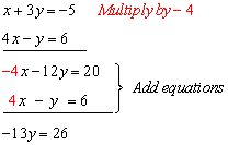
Look at the x - coefficients. Multiply the first equation by -4, to set up the x-coefficients to cancel.

Now we can find: y = -2

Take the value for y and substitute it back into either one of the original equations.

The solution is (x, y) = (1, -2).

Example 3: Solve the system using elimination method

Solution:

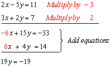
In this example, we will multiply the first row by -3 and the second row by 2; then we will add down as before.

Now we can find: y = -1

Substitute y = -1 back into first equation:

The solution is (x, y) = (3, -1).

Matrix

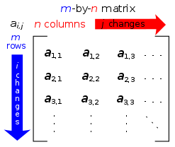
Matrix- is a rectangular array of numbers, symbols, or expressions, arranged in rows and columns.
A matrix with m rows and n columns is called an m × n matrix or m-by-n matrix, while m and n are called its dimensions.

Elements or Entries- individual items in a matrix 

 2 rows and 3 columns or 2 by 3



Matrix Multiplication-two matrices can be multiplied only when the number of columns in the first equals the number of rows in the second.

Row Vectors-Matrices which have a single row

Column Vectors-Matrices which have  a single column 

Square Matrix-matrix which has the same number of rows and columns 

Infinite Matrix-matrix with an infinite number of rows or columns (or both)

Introduction

POINT

x-3=0

LINE

x+3y=1

NON LINEAR EQUATION
xy+2=4

PLANE

2x-3y+2=1

LINEAR EQUATION

-1 example for every term

Types of Solution

1. Consistent

2. Inconsistent

PARAMETER
- specific sample out of the population

CONSISTENT Sample

1 solution

x+y=2

x-y=1

Infinite Solution

2x+2y=2

4x+4y=4

INCONSISTENT Sample

x+y=5

x+y=7

To limit the infinite solution

ex.

x1+2x2=4

x1= 4-2x2

x2= t, t is a whole number

x1= 4-2t

Linear Algebra

Linear algebra is the branch of mathematics concerning vector spaces and linear mappings between such spaces. It is the study of lines, planes, and subspaces and their intersections using algebra.